Ever felt overwhelmed when faced with massive datasets? You're not alone. In today's data-driven world, knowing how to efficiently extract and analyze information is a superpower. Welcome to the second lesson of BigQuery for Looker Studio, where we'll demystify SQL (Structured Query Language) and explore how it can transform your data analysis workflow.

By the end of this guide, you'll have the essential SQL skills to confidently query datasets and even use AI tools to supercharge your workflow. Let's jump into the world of structured queries!

What is SQL and Why Does it Matter?

SQL (pronounced "sequel" or "S-Q-L") stands for Structured Query Language. It's one of the most accessible programming languages in computer science, designed specifically for a single purpose: asking questions of a database.

Think of SQL as a translator between you and your data. When you have questions like "Which products generated the most revenue last month?" or "Where are my most valuable customers located?", SQL provides the language to ask these questions directly to your database.

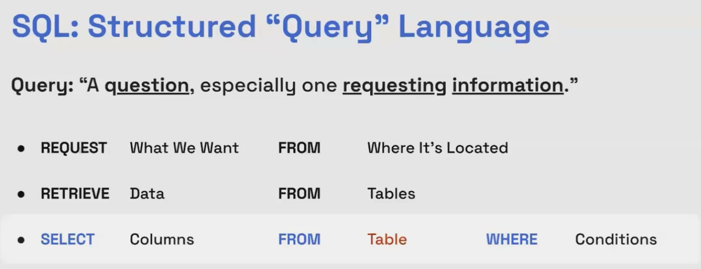
The "Query" in SQL refers to the process of requesting specific information from your database. It's like having a conversation with your data where you specify:

What information you want (SELECT)
Where that information is located (FROM)
Which conditions the data should meet (WHERE)

The Basic Structure of SQL

At its most fundamental level, SQL follows this pattern:

SELECT columns_you_want
FROM table_where_data_lives
WHERE conditions_are_met

This simple structure is powerful enough to handle most of your data retrieval needs. As of 2025, BigQuery continues to enhance its SQL capabilities with the latest being the MATCH_RECOGNIZE clause for advanced pattern matching across rows, but the core syntax remains consistent.

Understanding Tables: The Building Blocks of SQL

Before diving deeper into SQL commands, let's understand what we're querying: tables.

In the world of SQL, data is organized into tables consisting of rows and columns – similar to spreadsheets but with more structure:

Columns represent fields or attributes (like 'First_Name', 'Revenue', 'Order_Date')
Rows contain the actual data entries corresponding to those fields

For our examples, we'll use a sample dataset for an online store with information about customers, orders, products, and revenue.

Database tables organize data into columns (fields) and rows (records), creating a structured framework for queries.

Importing Your Data into BigQuery

Before writing queries, we need data in BigQuery. One of the simplest approaches is importing from Google Sheets:

Navigate to your BigQuery project
Click the three-dot menu beside your dataset and select Create table
Select Drive as your source and paste your Google Sheet URL
Name your table (e.g., online_store_orders)
Choose External table as the table type
Enable Auto-detect for schema detection
Check "Header rows to skip" and set it to 1
Click Create table

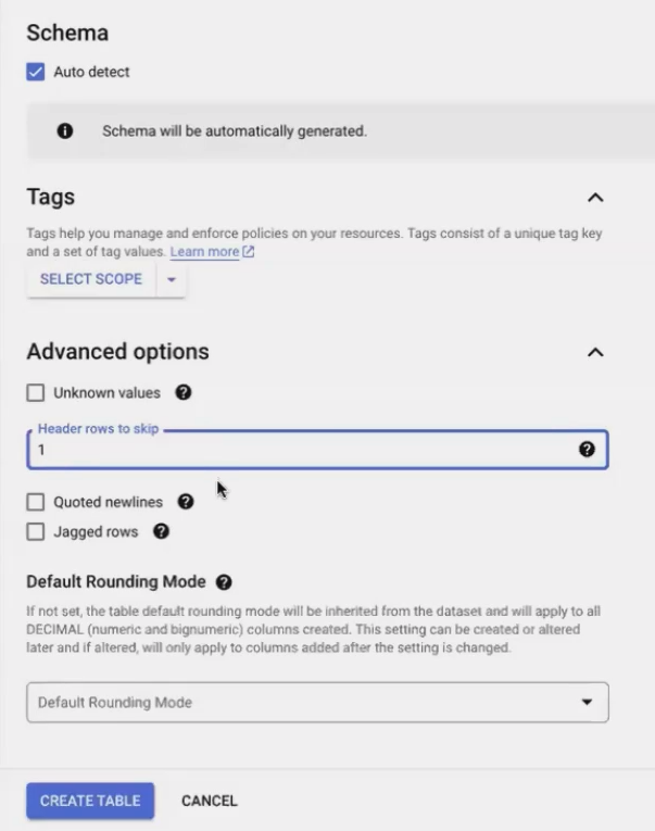
Creating an external table means BigQuery will reference data directly from your Google Sheet. Any updates to the sheet will automatically appear in your queries – perfect for maintaining a single source of truth!

Essential SQL Commands for Data Analysis

Let's explore the core SQL commands that will handle 80% of your data analysis needs:

1. The SELECT Command: Choosing Your Data

The SELECT statement is where every query begins. It specifies exactly which data you want to retrieve.

Selecting Static Values:

SELECT 
  "Siavash" AS instructor_name, 
  92.5 AS certification_score

This creates two columns with the specified values. The AS keyword creates an "alias" – a user-friendly name for your columns.

Selecting Columns from a Table:

SELECT
  order_date,
  customer_id,
  revenue
FROM
  `project_name.dataset_name.online_store_orders`

This retrieves just the specified columns from your table. To select all columns, use the wildcard character:

SELECT * 
FROM `project_name.dataset_name.online_store_orders`

2. Filtering with the WHERE Clause

The WHERE clause is where your analysis gains focus – it filters data to include only rows that meet specific conditions.

Basic Filtering:

SELECT
  first_name,
  last_name,
  state
FROM
  `project_name.dataset_name.online_store_orders`
WHERE
  state = "New York"

Using Multiple Conditions:

SELECT * 
FROM `project_name.dataset_name.online_store_orders`
WHERE 
  (state = "New York" AND channel = "Direct") 
  OR product = "Jump Rope"

Handling NULL Values:

SELECT * 
FROM `project_name.dataset_name.online_store_orders`
WHERE first_name IS NOT NULL

Remember that null values require special operators (IS NULL or IS NOT NULL) – using equals (=) won't work!

3. Sorting Results with ORDER BY

The ORDER BY clause lets you arrange your results in a meaningful sequence:

SELECT * 
FROM `project_name.dataset_name.online_store_orders`
ORDER BY 
  order_date DESC,  -- Most recent orders first
  revenue DESC   --  Highest revenue orders at the top for each date

Add DESC for descending order (highest to lowest, newest to oldest); the default is ASC (ascending).

4. Limiting Results with LIMIT

The LIMIT clause restricts the number of rows returned:

SELECT * 
FROM `project_name.dataset_name.online_store_orders`
ORDER BY order_date DESC
LIMIT 5  -- Only return the 5 most recent orders

This is particularly useful during data exploration when you don't need to process the entire dataset.

5. Finding Unique Values with DISTINCT

The DISTINCT keyword removes duplicates from your results:

SELECT DISTINCT
  state
FROM
  `project_name.dataset_name.online_store_orders`

This shows you exactly which states appear in your data, with each state listed only once.

Transforming Data with Calculations and Functions

SQL isn't just for retrieving data – it's also for transforming it into more useful forms.

Creating Calculated Fields

You can perform calculations and apply functions to create new values:

Numeric Calculations:

SELECT
  order_id,
  revenue,
  revenue * 0.25 AS profit  -- Assuming 25% profit margin
FROM
  `project_name.dataset_name.online_store_orders`

Text Manipulation:

SELECT
  INITCAP(first_name) AS properly_formatted_first_name,  -- Capitalizes first letter
  CONCAT(INITCAP(first_name), " ", INITCAP(last_name)) AS full_name
FROM
  `project_name.dataset_name.online_store_orders`

BigQuery offers dozens of built-in functions for manipulating text, dates, and numbers. The INITCAP function (added in recent versions) is particularly useful for standardizing names by capitalizing the first letter of each word.

Aggregating Data for Insights

Aggregation is where SQL truly shines for analysis – it allows you to summarize data across multiple rows.

Basic Aggregation Functions

Common aggregation functions include:

COUNT(): Counts the number of rows
SUM(): Adds up values
AVG(): Calculates the average
MAX() and MIN(): Find the highest and lowest values

SELECT
  COUNT(*) AS number_of_orders,
  COUNT(DISTINCT customer_id) AS number_of_customers,
  SUM(revenue) AS total_revenue,
  AVG(revenue) AS average_order_value,
  MAX(revenue) AS largest_order
FROM
  `project_name.dataset_name.online_store_orders`

Grouping Data with GROUP BY

The real power comes when you combine aggregations with the GROUP BY clause to analyze segments of your data:

SELECT
  state,
  COUNT(*) AS orders_count,
  SUM(revenue) AS total_revenue,
  AVG(revenue) AS average_order_value
FROM
  `project_name.dataset_name.online_store_orders`
GROUP BY
  state
ORDER BY
  total_revenue DESC

This query shows you performance metrics for each state, sorted by total revenue.

The Golden Rule of GROUP BY: Every column in your SELECT statement must either be:

Included in the GROUP BY clause, OR
Used within an aggregate function (like SUM, COUNT, etc.)

You can group by multiple columns to create more specific segments:

SELECT
  state,
  city,
  COUNT(*) AS orders_count,
  SUM(revenue) AS total_revenue
FROM
  `project_name.dataset_name.online_store_orders`
GROUP BY
  state, city

Putting It All Together: Customer Analysis Example

Let's combine everything we've learned to build a comprehensive customer analysis table:

SELECT
  customer_id,
  CONCAT(INITCAP(first_name), ' ', INITCAP(last_name)) AS customer_name,
  state AS customer_state,
  city AS customer_city,
  
  -- Lifetime value metrics
  SUM(revenue) AS customer_ltv,
  AVG(revenue) AS customer_aov,
  COUNT(DISTINCT order_id) AS frequency,
  
  -- Customer timeline metrics
  MIN(order_date) AS first_order_date,
  MAX(order_date) AS last_order_date,
  DATE_DIFF(CURRENT_DATE(), MIN(order_date), DAY) AS customer_age_days,
  DATE_DIFF(CURRENT_DATE(), MAX(order_date), DAY) AS recency_days
FROM
  `project_name.dataset_name.online_store_orders`
GROUP BY
  customer_id, customer_name, customer_state, customer_city
ORDER BY
  customer_ltv DESC

This query:

Cleans and formats customer information
Calculates key metrics like lifetime value and purchase frequency
Determines when customers first and last purchased
Measures customer age and recency
Orders results to show highest-value customers first

Once you have this query result, BigQuery offers a fantastic feature: Explore with Looker Studio. Clicking this button instantly connects your query results to a new Looker Studio report for immediate visualization!

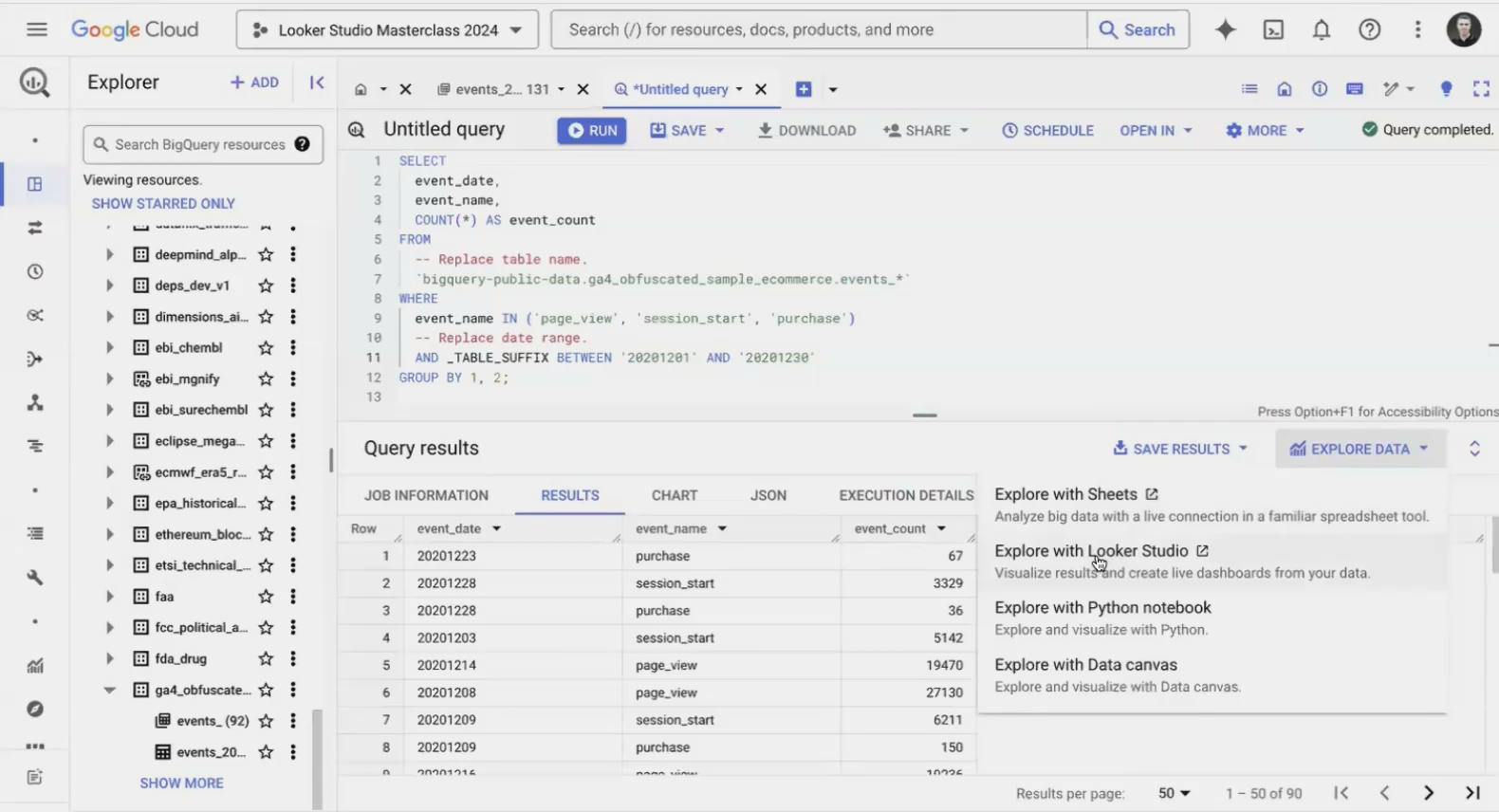
The "Explore with Looker Studio" button bridges the gap between SQL queries and visual analysis.

Frequently Asked Questions (FAQs)

What's the practical use case for limiting rows with the LIMIT command?

While LIMIT rarely appears in production queries, it's invaluable during development. It lets you quickly preview results without processing the entire dataset (saving time and computational resources), provides manageable samples for testing, and creates small data extracts for sharing with colleagues or AI tools.

Can I use column aliases in calculations within the same SELECT statement?

In BigQuery SQL, you cannot reference an alias created in the same SELECT clause. For example, if you create SUM(revenue) AS total_revenue, you cannot use total_revenue in another calculation within that same SELECT statement. To build upon previous calculations, you'll need to use subqueries or Common Table Expressions (CTEs), which we'll cover in future lessons.

When using GROUP BY, do I still need DISTINCT?

Generally, no. The GROUP BY clause inherently consolidates all matching rows into a single result row. For example, if "California" appears in 500 rows, GROUP BY state will produce just one row for "California." There's no need for DISTINCT on columns you're grouping by.

Are there any size limitations when connecting BigQuery to Looker Studio?

There are no restrictions on the size of BigQuery tables you can connect to Looker Studio. Looker Studio is optimized to push computational work back to BigQuery, retrieving only the aggregated data needed for visualization. However, individual visualizations have practical limits – for instance, a table chart might display only the first 200,000 rows.

If you're ready to take your SQL skills to the next level, these free resources are excellent next steps:

Mode Analytics SQL Tutorial: Comprehensive lessons with real-world examples
W3Schools SQL Course: Interactive exercises to practice core concepts
Google's BigQuery Documentation: Detailed reference for BigQuery-specific features

As of 2025, SQL remains one of the most in-demand technical skills, with the ability to query and analyze data continuing to be essential across industries. The newest additions to BigQuery's SQL capabilities include the MATCH_RECOGNIZE clause for pattern matching across rows and enhanced pipe syntax for more readable queries, making SQL even more powerful for complex analysis.

Remember that mastering SQL is a journey – start with these essentials, practice regularly with real data, and gradually incorporate more advanced techniques as you become comfortable. The foundation you've built today will serve you throughout your data analysis career!

Note:

This post is based on a subject covered in the Looker Studio Masterclass Program. To learn more about Looker Studio Masterclass, click here.

Essential SQL Commands for BigQuery: Transform Raw Data into Actionable Insights